One of the most critical aspects of model development is ensuring that our models can generalize well to unseen data (i.e. when the predictions are deployed). While it's relatively straightforward to train a model that performs well on training data, the real challenge is creating models that maintain their performance when faced with new, previously unseen examples. This is where cross-validation (CV) comes into play to validate our models' performance and make more informed decisions during the model development process. Throughout this post, we will review different CV variants and how Faraday uses them to train its model and forecast return on investment (ROI) for our clients.

What is cross-validation

At its core, cross-validation is a resampling procedure used to evaluate machine learning models on limited data samples. Instead of using a single train-test split, cross-validation provides a framework for multiple evaluations of our model using different portions of the available data.

Cross-validation involves partitioning the available data into complementary subsets, training the model on some subsets (training set), and validating it on the remaining subset (validation set). This process is repeated multiple times, with each data point getting the opportunity to be part of both training and validation sets.

The key principles of cross-validation include:

1. Data Independence: Ensuring that training and validation sets are strictly separated in each iteration
2. Comprehensive Evaluation: Using all available data for both training and validation through multiple iterations
3. Statistical Robustness: Generating multiple performance metrics to assess model stability

K-Fold cross-validation

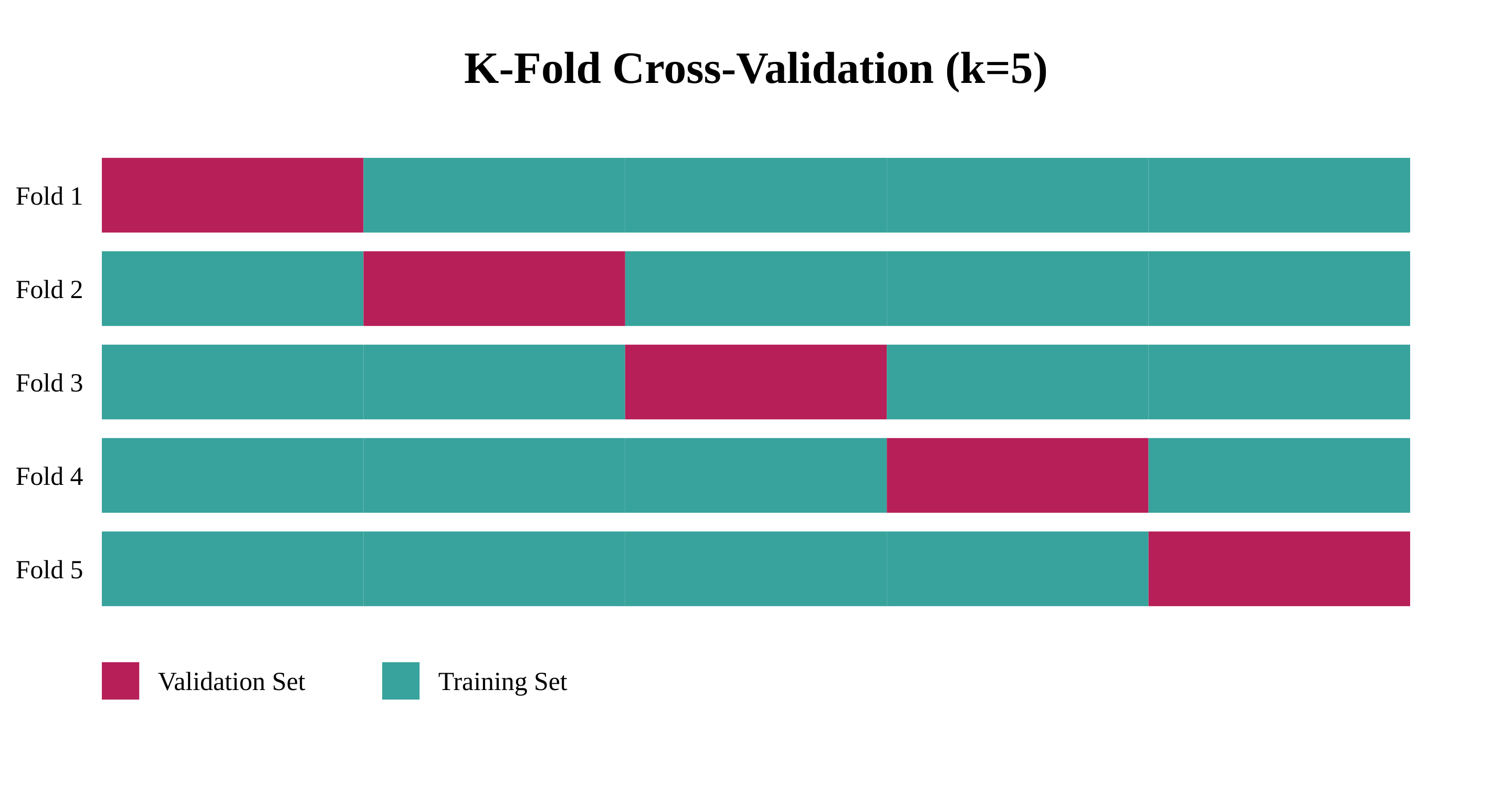
K-fold cross-validation is the most common and widely used variant of cross-validation. In this approach, the data is divided into k equal-sized folds, and the following process is repeated k times:

1. One fold is selected as the validation set
2. The remaining k-1 folds are used as the training set
3. One model is trained on the training set
4. Predictions on the validation set are saved

Faraday uses a 5-fold CV to evaluate its models. This means that for any given propensity model, Faraday builds 6 variations of the model (5 for the k-fold validation and one final version used as the deployed model.)

Once all five models are trained, each sample in the data has been scored once. This means that the cross-validation allows us to assign a prediction to each person, allowing us to compute the performance metrics using the reconstructed scores.

Special variants of k-fold cross-validation include:

• Stratified K-Fold: Maintains the same class distribution in each fold (useful for imbalanced datasets)
• Leave-one-out cross-validation: Sets k equal to the number of data points (useful for very small datasets)
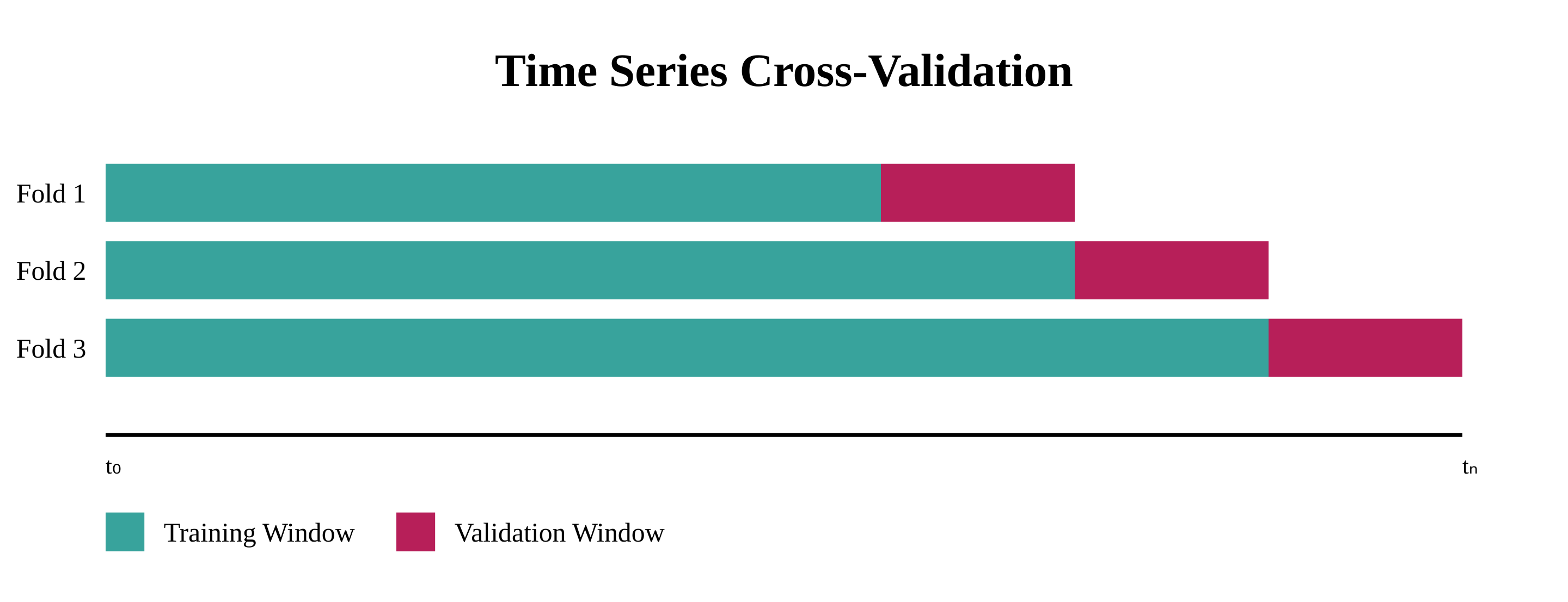
• Time series cross-validation: The folds are defined using a rolling window for time-based data.

The benefits of cross-validation

From the previous section, it is clear that CV implies more computation than training a single model. However, cross-validation offers several crucial advantages that outweigh the added costs and complexity, making it a mandatory step in the training process. Let's explore the key benefits that make this technique so valuable.

Preventing overfitting

One of the primary benefits of cross-validation is its ability to help prevent overfitting. When a model learns the training data too well, it starts to capture noise and specific patterns that don't generalize to new data. Overfitting leads to poor performance in real-world applications. In the charts below, we compare the effects of three different model architectures on the same dataset:

1. The first model is too simplistic to capture the trend in the data.
2. The third one tries too hard to capture every data point and adds a lot of noise between them.
3. The second model does a good job of capturing the overall trend in the data without necessarily trying to capture small variations in the location of the data points.

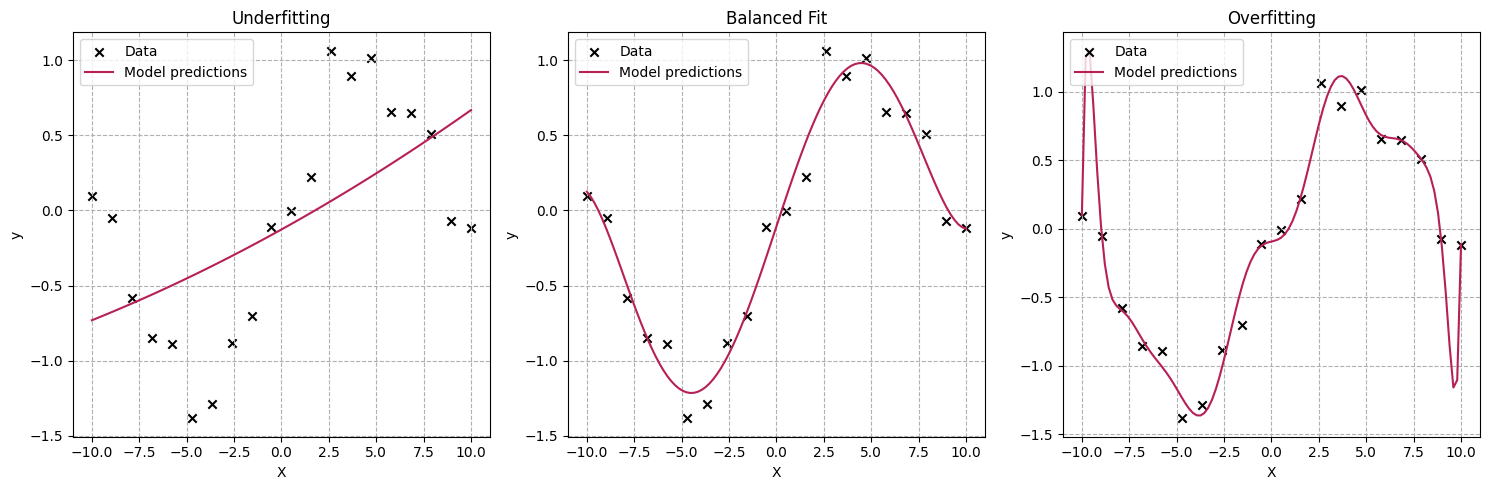
Cross-validation helps detect overfitting by evaluating the model's performance on multiple subsets of the data. If a model performs significantly better on the training data than on the validation sets, it's a clear indicator of overfitting. This early detection allows data scientists to make necessary adjustments to the model's complexity, feature selection, or hyperparameters before deploying it to production.

If we compute our model performance (ROC, accuracy) on the training data, the third model is the best option. However, when using CV, the second model performs better.

Computing reliable performance metrics

Traditional train-test splits can sometimes provide misleading performance metrics due to the random nature of the split. Cross-validation addresses this limitation by:

• Providing multiple performance estimates using different data splits
• Enabling the calculation of confidence intervals for performance metrics
• Reducing the variance in performance estimation
• Offering a more robust assessment of model stability

These multiple evaluations give us a clearer picture of how our model is likely to perform in real-world scenarios, helping us make more informed decisions about model selection and deployment.

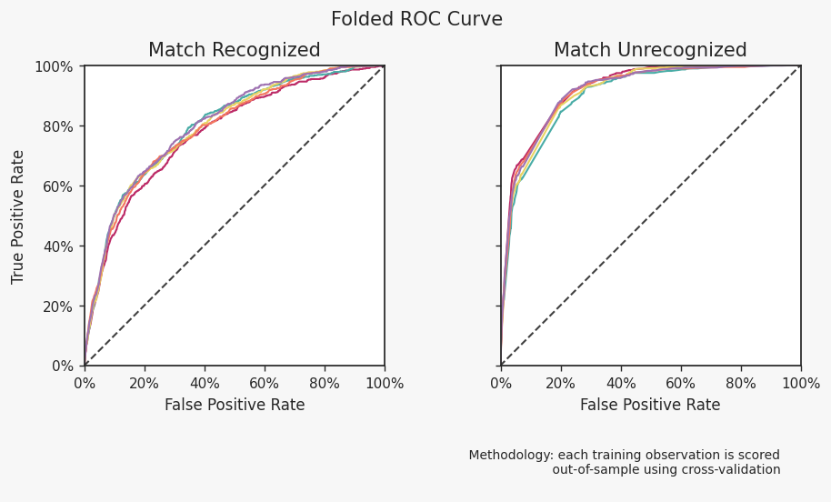
The content of our outcome report and UI relies entirely on the cross-validation but two charts explicitly depict results per fold. Our “folded ROC” plot shows the ROC curve for each fold. This is useful to ensure the model is stable (i.e. the results across folds are nearly identical).

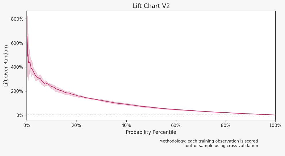
The lift chart illustrates the volatility of lift, particularly for those with higher scores. This information is crucial for lead generation models, which aim to identify potential customers. Faraday assigns a score to each individual within a specified population, and the client uses only the top X% of scorers.

Technical dive

Formal definitions

Dataset definition

• Let $\mathcal{D} = \{(x_i, y_i)\}_{i=1}^n$ be our dataset where:
• $x_i \in \mathcal{X} \subseteq \mathbb{R}^d$ are feature vectors for sample $i$
• $y_i \in \mathcal{Y}$ is the label for sample $i$
• $n$ is the number of samples
• Define $\mathcal{P}_{XY}$ as the true joint distribution of $(X,Y)$

Model space

• Let $\mathcal{F} = \{f_\theta: \mathcal{X} \rightarrow \mathcal{Y} | \theta \in \Theta\}$ be the hypothesis space
• $\theta$ represents the model parameters
• $\Theta$ is the parameter space

Loss function

• Define $\mathcal{L}: \mathcal{Y} \times \mathcal{Y} \rightarrow \mathbb{R}_{\geq 0}$ as the loss function
• The expected risk is:

$$R(f) = \mathbb{E}_{(X,Y)\sim\mathcal{P}_{XY}}[\mathcal{L}(f(X),Y)]$$

$R(f)$ is interpreted as the error of the model $f$ on the dataset.

• The empirical risk on dataset $\mathcal{D}$ is the average loss over $\mathcal{D}$:

$$\hat{R}_{\mathcal{D}}(f) = \frac{1}{n}\sum_{i=1}^n \mathcal{L}(f(x_i),y_i)$$

K-Fold partitioning

• Partition indices $\{1,\ldots,n\}$ into $k$ disjoint subsets: $\{\mathcal{I}_1,\ldots,\mathcal{I}_k\}$
• For each fold $j$:
  • $\mathcal{D}_{val}^{(j)} = \{(x_i,y_i) | i \in \mathcal{I}_j\}$ (validation set)
  • $\mathcal{D}_{train}^{(j)} = \{(x_i,y_i) | i \notin \mathcal{I}_j\}$ (training set)

Cross-validation estimator
The k-fold CV estimate of the expected risk is:

$$CV_{(k)}(f) = \frac{1}{k}\sum_{j=1}^k \hat{R}_{\mathcal{D}_{val}^{(j)}}(f_{\theta_j})$$

where $f_{\theta_j}$ is trained on $\mathcal{D}_{train}^{(j)}$

Statistical properties

Bias of CV estimator
The bias of the k-fold CV estimator can be expressed as:

$$Bias(CV_{(k)}) = \mathbb{E}[CV_{(k)}] - R(f^*)$$

where $f^*$ is the true optimal function and $\mathbb{E}[CV_{(k)}]$ is the expected risk over all the folds.

Variance decomposition
The variance can be decomposed into:

$$Var(CV_{(k)}) = \frac{1}{k^2}\sum_{j=1}^k Var(\hat{R}_{\mathcal{D}_{val}^{(j)}}) + \frac{2}{k^2}\sum_{i<j}Cov(\hat{R}_{\mathcal{D}_{val}^{(i)}}, \hat{R}_{\mathcal{D}_{val}^{(j)}})$$

Where $Var(\hat{R}_{\mathcal{D}_{val}^{(j)}})$ is the variance of the risk estimate over a fold. It does not refer to the variance of the risk itself (which is just a scalar value). Instead, it refers to the variance of the estimated risk based on multiple possible samples of the validation set within that fold.

Therefore, as k increases, the overall variance of the cross-validation risk decreases leading to a less volatile estimation of the model performance post-deployment.

Holdout test

What is it?

A "holdout test" can refer to any process where a model is being evaluated on unseen data (e.g. cross-validation above). At Faraday, a holdout test specifically refers to the process of choosing a date in the past $t_0$, fitting a propensity model with data prior to $t_0$, and evaluating the model on data after $t_0$.

On one hand, a holdout test is just a special case of time series cross-validation with 1 fold, but as we will see there are a few nuances to consider when configuring a holdout test and analyzing the results to inform a business decision.

Configuring a holdout test in the Faraday platform

A typical scenario where a holdout test can be used is lead scoring. We will walk through how to run a lead scoring holdout test in the Faraday platform, but the same principles apply to a holdout test for other use-cases (e.g. predicting churn).

What is needed for a holdout test?

To configure a holdout test a user needs lead and conversion records with PII, dates, and a way to distinguish between the two groups. The setup for this can vary, but perhaps the simplest form is a single table that includes the following:

• PII columns
• a lead_created date that captures when a record became a lead
• a conversion_date that captures when that lead record became a conversion

NOTE: In our working example our conversions are called tier_1_leads.

In addition to the raw data, a user needs to have some prior knowledge of the typical attribution window for conversion which we will discuss in more detail when configuring the cohorts.

Datasets and events

Given a dataset described above, we need to configure the PII as one or more identity sets and two event streams, one for leads and one for conversions.

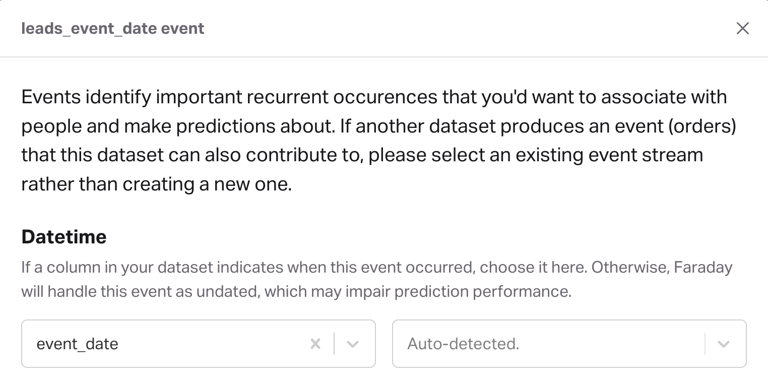
Configuring the leads event can be as simple as mapping a single date column

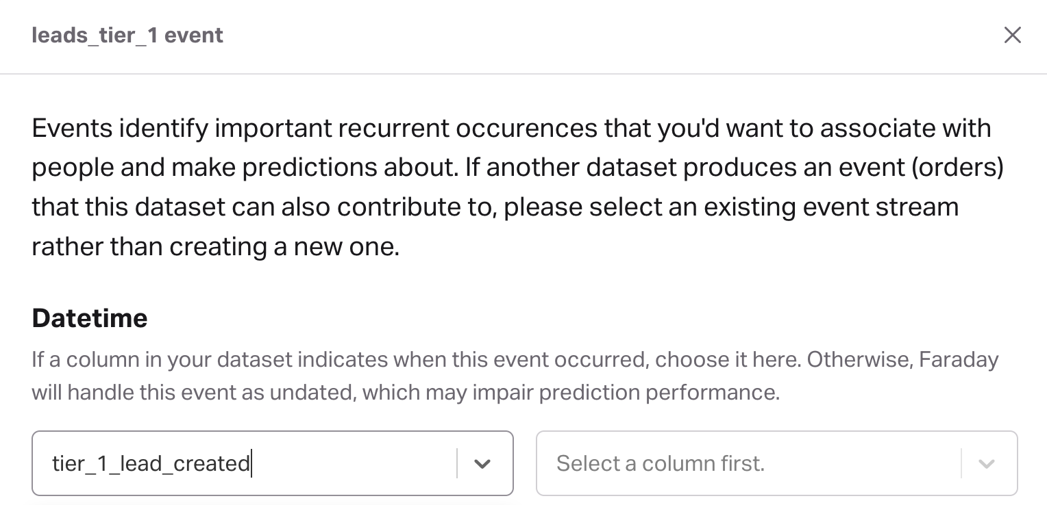
Similarly for the tier_1_leads event

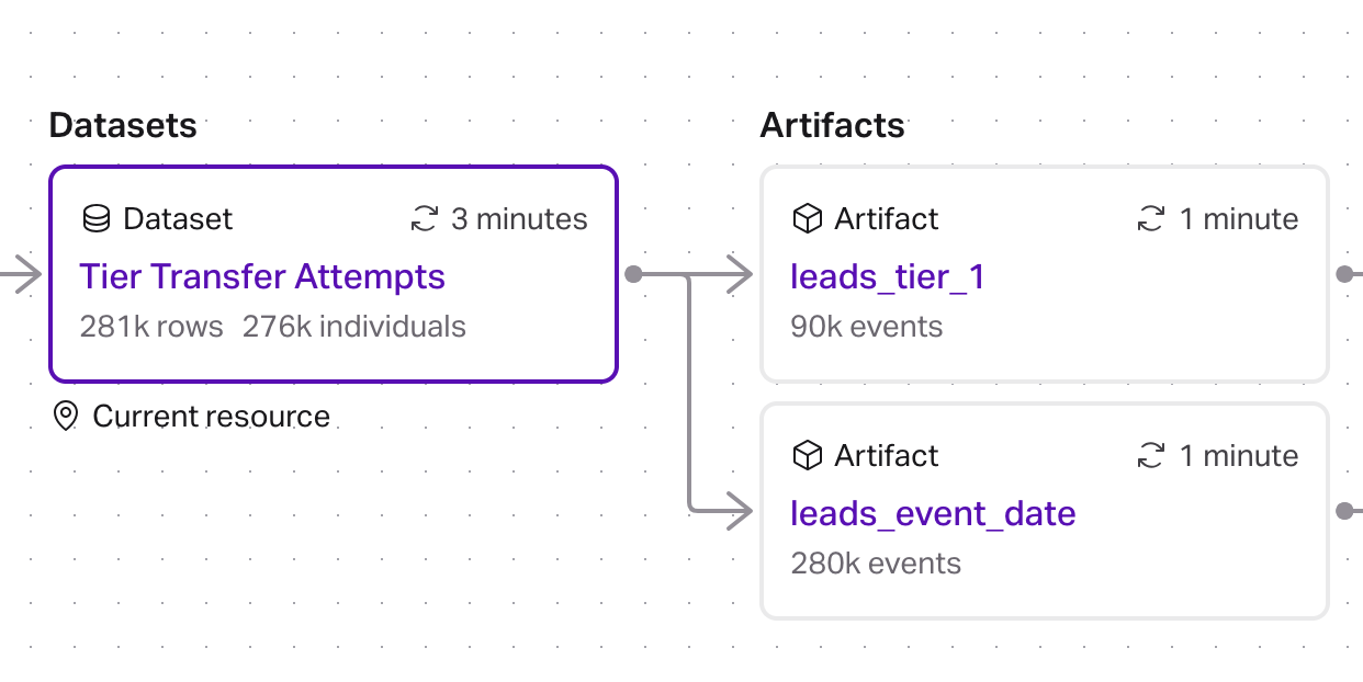
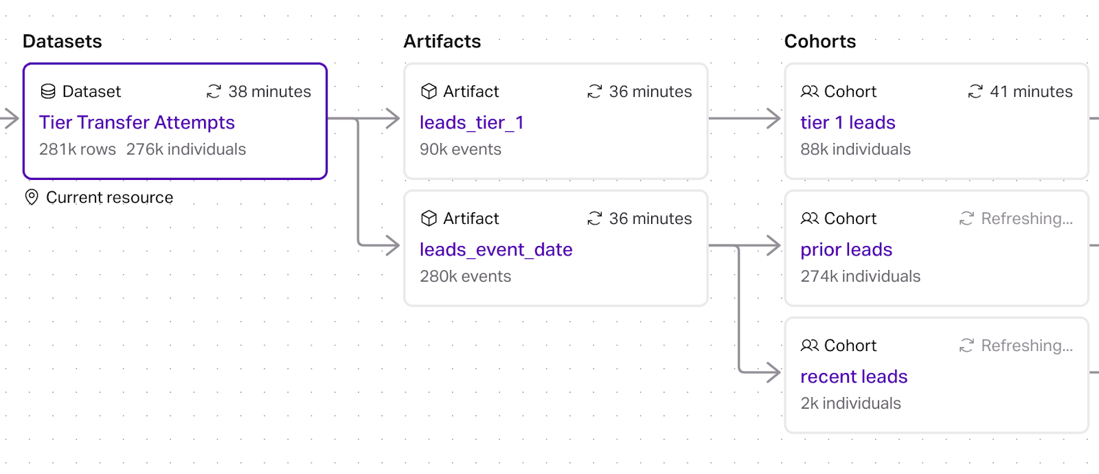
At this point our resource graph has a dataset table that emits two event streams

Cohorts

Next, we need to configure groups of people (cohorts) that partition the data into a training and validation set (recall this is time series cross-validation with 1 fold).

The inputs to determine this are:

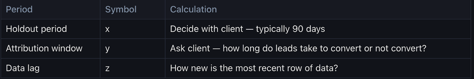
The "prior period" is the training set for the holdout test, and the "holdout period" is the validation set. The amount of data available can influence how long/short these time windows are, but in general, we want to have enough data in the prior period to train a model and enough data in the holdout period to be confident in the results. For example, it would be bad to have zero conversions in the holdout period.

The attribution window is the time it takes for a typical lead to convert. Depending on the situation, this could be a few days to months.

The data lag is the time delta between today and the most recent date of any lead or conversion.

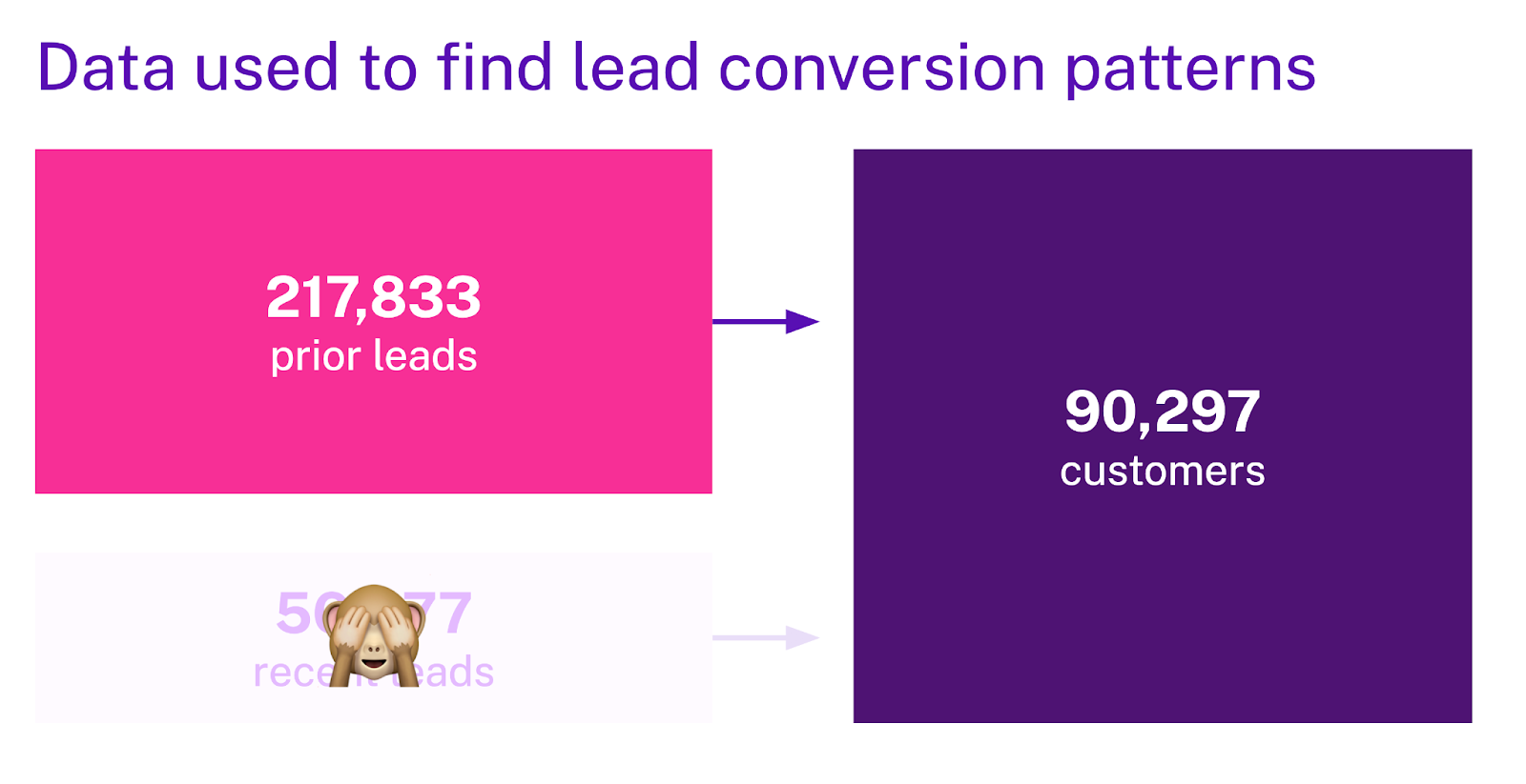
Once these have been determined we can create three cohorts

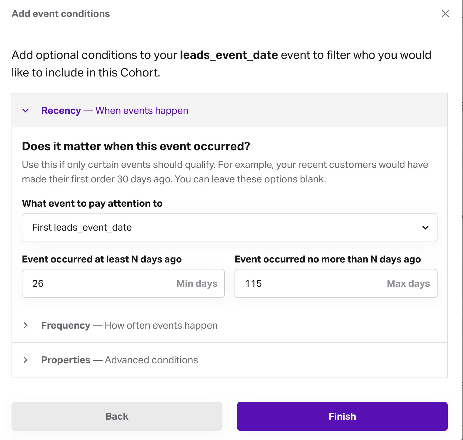
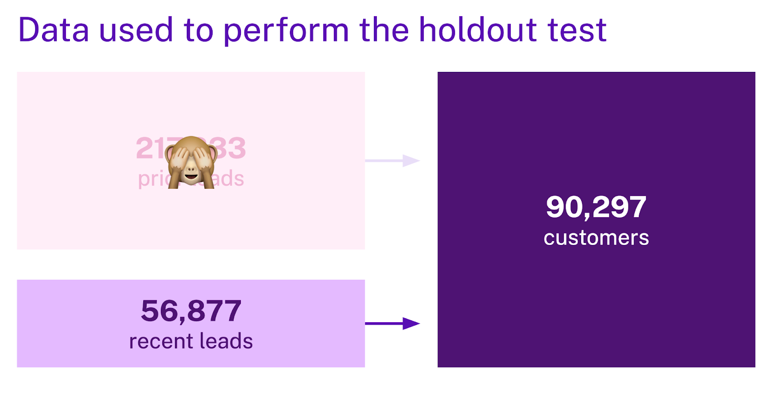
• prior leads: all records that became leads in the prior period
• recent leads: all records that became leads after the prior period
• conversions: all conversions (tier_1_leads in the working example) without any date filtering

Prior leads example configuration

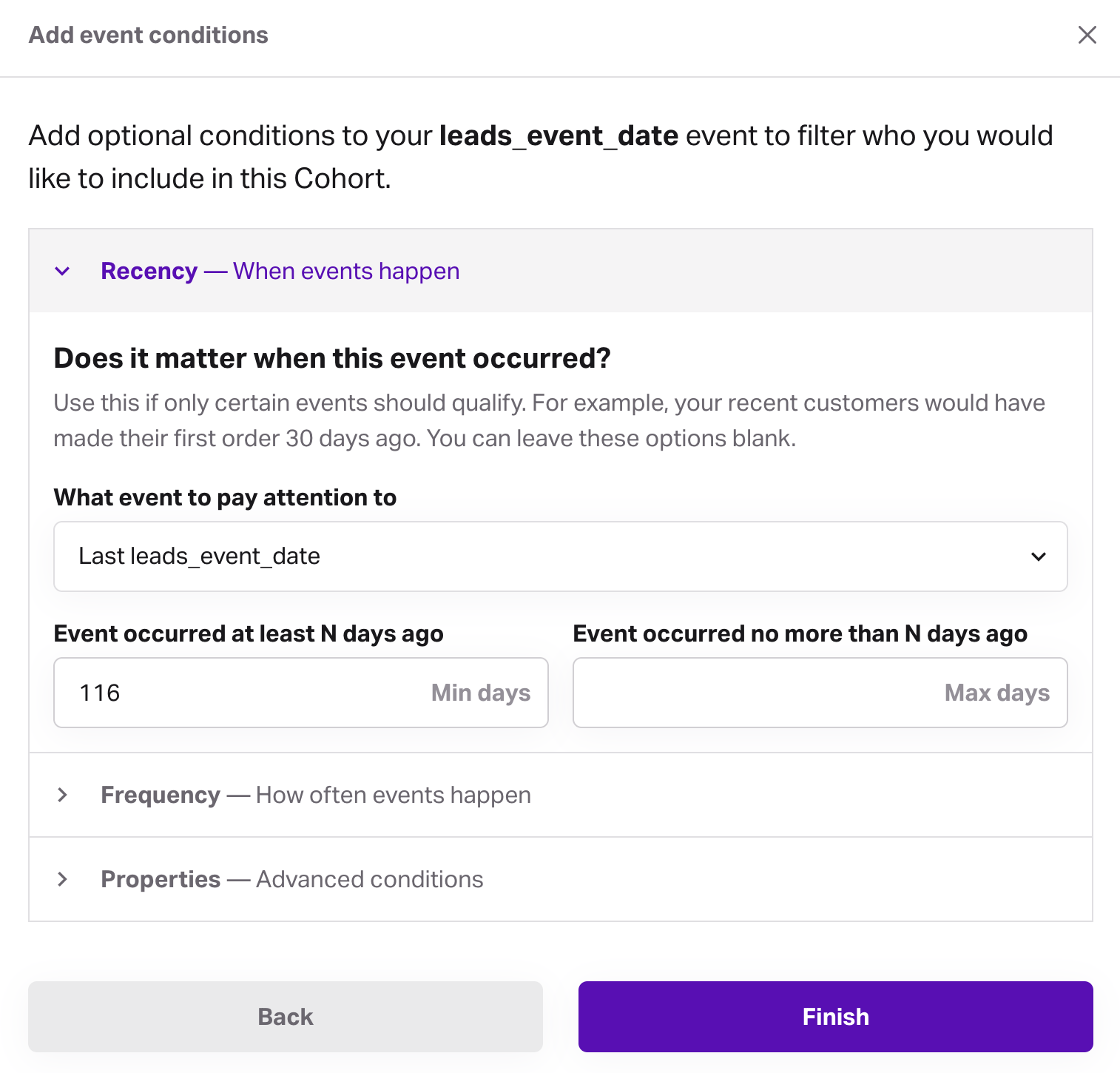
Recent leads example configuration

Our resource graph now looks like

Outcome

Once cohorts are configured it is time to build a model and get some output. In Faraday, a propensity model is defined by an "outcome" which takes two cohorts as an input.

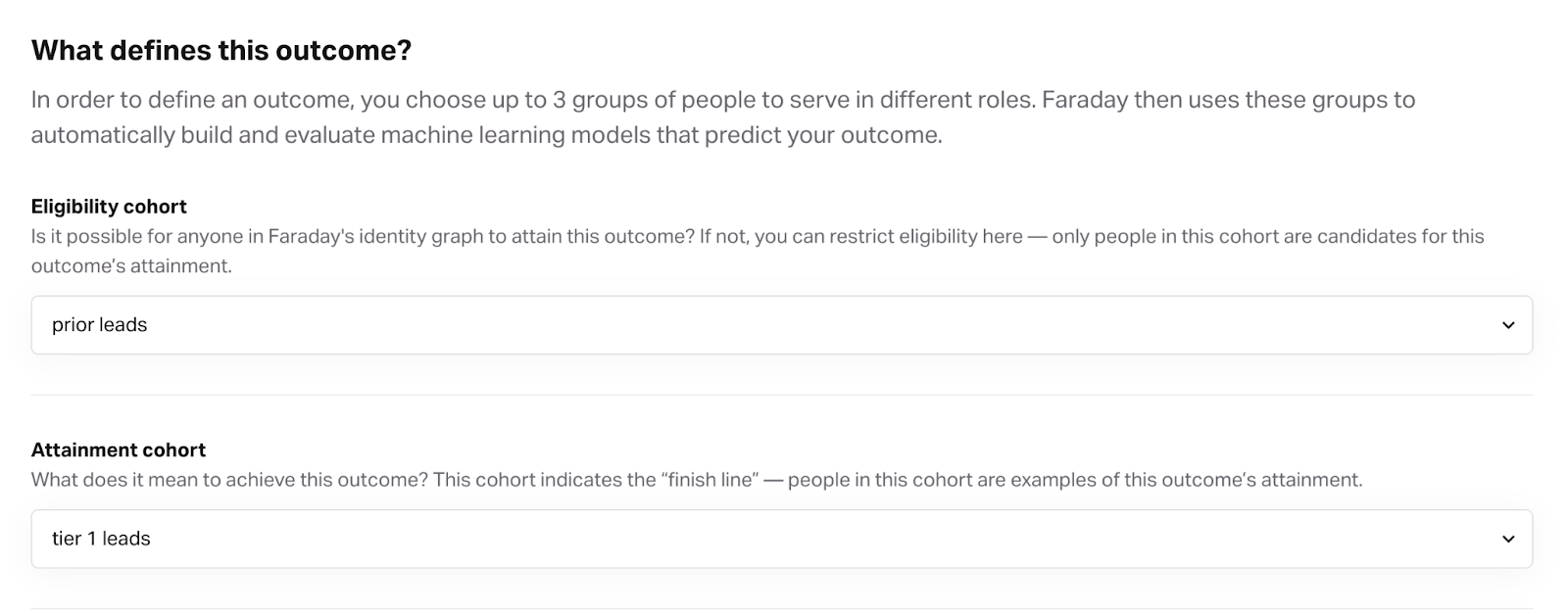
Note that using the prior leads from the prior period implicitly restricts the conversions (tier 1 leads) to the prior period.

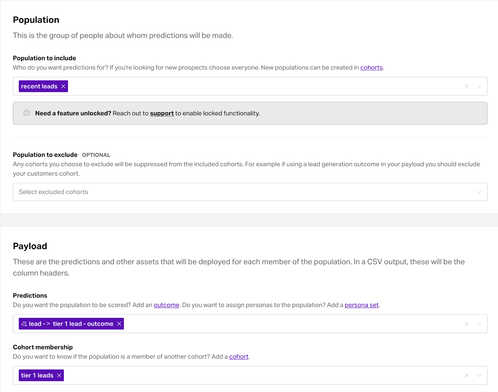
Pipeline

A pipeline applies an outcome (propensity model) to a group of people specified by a cohort. In this case we want to apply the outcome trained using data from the prior period to score recent leads records. Additionally, we want to have conversion information available in the output to analyze performance.

Here is the full resource graph

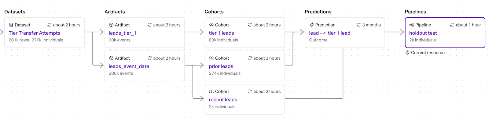
This pipeline produces a table whose rows correspond to the recent lead records and whose columns include:

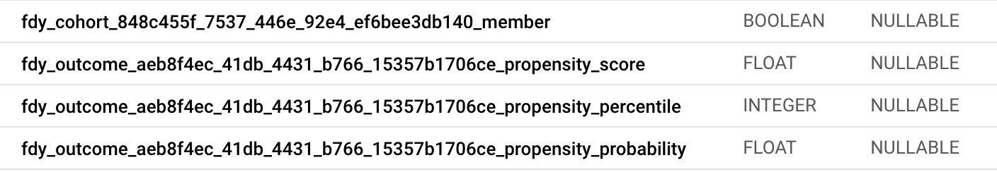
Any of the fdy_outcome_ columns can be used together with the fdy_cohort_*_member column (which is true when a row is a conversion) to measure model performance.

Analyzing results

The output from the above pipeline can be used for custom analysis as desired by the user. One example is the automated reporting that Faraday produces to analyze holdout results and potential ROI.

Holdout results

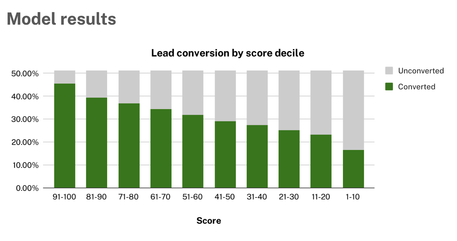
First, we look at the internal performance metrics of the model built using the prior period.

These metrics are based on cross-validation described above and distilled down into a single plot.

Next, we look at the pipeline output to see how the model performed on the recent leads.

Again, we can produce conversion rates by decile.

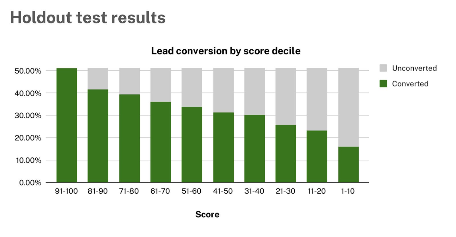
The last step of the holdout analysis is to compare the observed results from the holdout test with the model performance computed at training time via cross-validation.

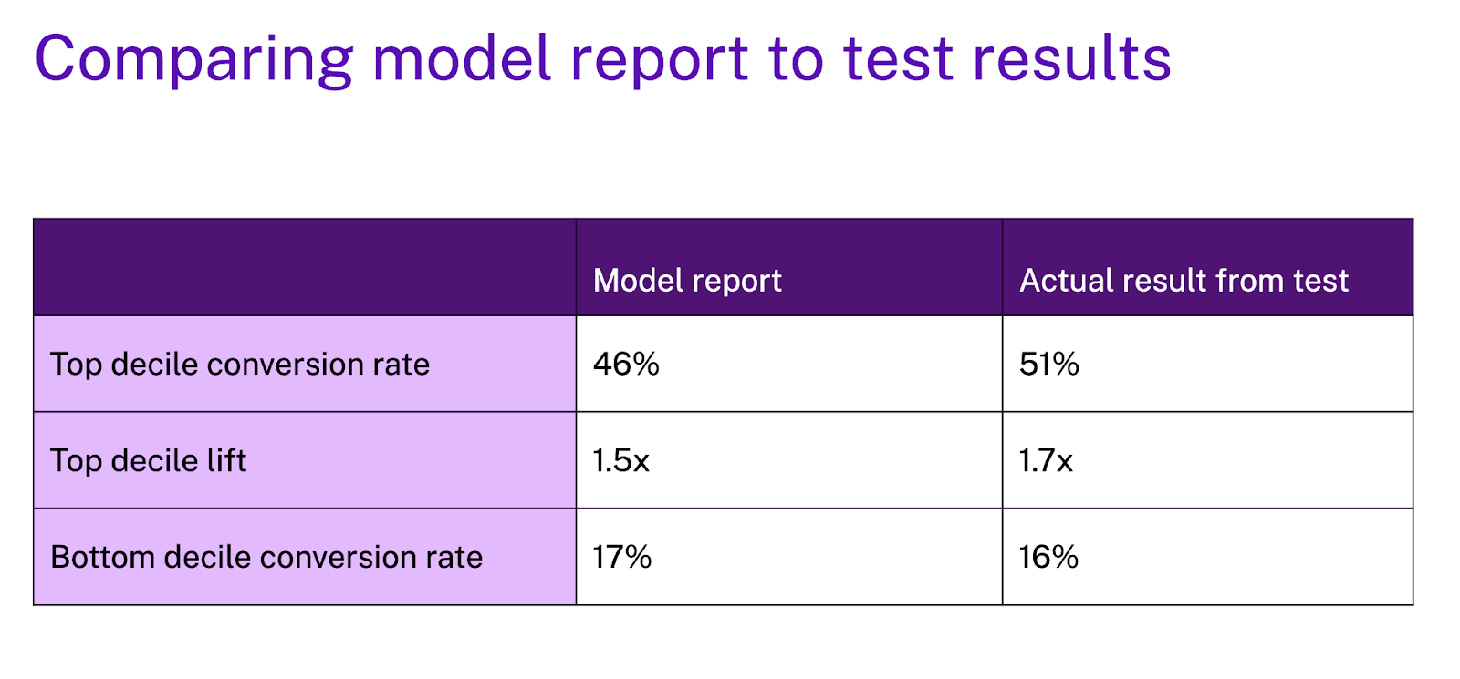
If these results are comparable, then it gives the user confidence that the performance metrics observed at training time are reflective of the model performance moving forward.

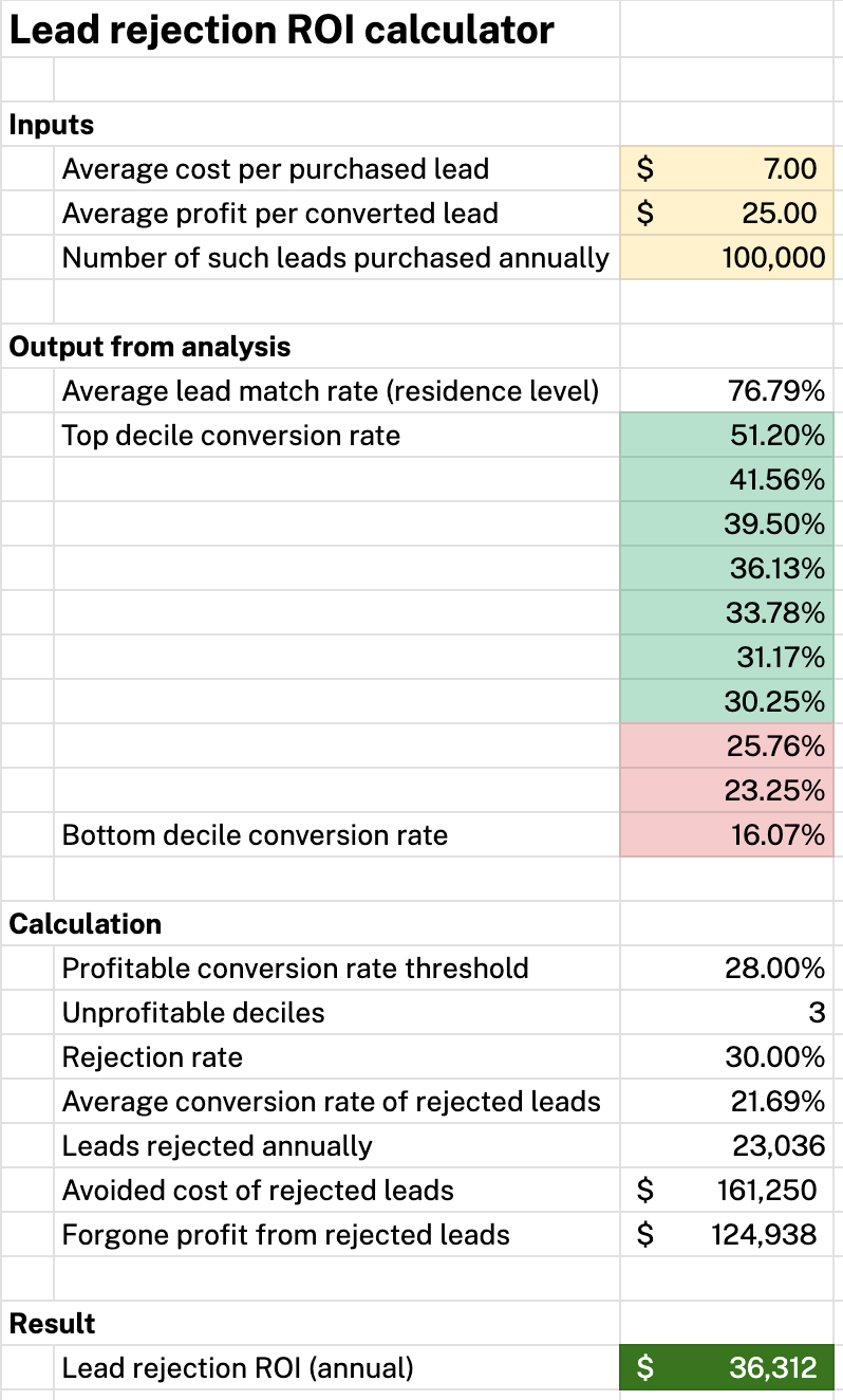
ROI calculation

When additional business context is known, the holdout test results can also be used to estimate ROI. For example

Conclusion

Cross-validation can be used to prevent overfitting and evaluate a model's performance at training time. A holdout test is just a special case of cross-validation in which a single fold is determined by a point in time. Combining these two approaches with business assumptions enables the user to deploy models confidently, with a sense of expected performance and insight into expected ROI.