Faraday bias reporting: How we measure & report on bias

What is bias?

Bias can rear its ugly head in various forms, from implicit biases that occur without the human actor being aware of it, to conscious bias in the inverse. While bias in data is historically more prevalent in certain B2C industries, like financial services, it doesn’t exclusively live there. With AI continuing its rise in popularity & use, the chance for bias to be propagated is high unless humans intervene and take steps to mitigate it in their data before it’s fed into machine learning algorithms.

One of Faraday’s founding pillars is the use of Responsible AI, which includes both preventing direct harmful bias and reporting on possible indirect bias. We recently announced the release of bias management tools in Faraday, and today we’re going to take a deep dive into the science behind Faraday’s bias reporting.

How to measure bias & fairness in AI

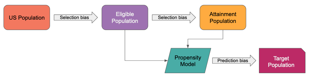
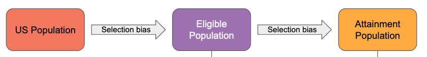
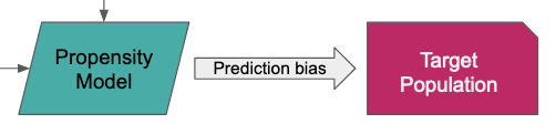
Faraday bias reporting aims to measure two types of bias inherent in the prediction pipeline: Selection bias in the determination of training sets, and prediction bias in the resulting scores/probabilities.

Quantifying bias in predictive modeling is an active research area. Survey papers, e.g. [1, 2], detail over 100 distinct metrics to measure bias and to define fairness in this context. Despite this variety, certain metrics appear to be used more commonly as the field evolves (see Table 10 in [2] and Table 1 in [6]).

Some background and notation

The following notation is fixed throughout the article.

$p$ is used to denote a probability distribution, $E$ for expectation, and $p(\cdot\mid\cdot)$ conditional probability.

Let $f: U\to[0,1]$ be a binary classifier mapping a feature vector $x$ to a score $f(x)$ in the unit interval. By encoding the coordinates of $x$ we can assume that $U$ is a subset of Euclidean space.

Let $y$ denote the ground-truth label of $x$. Let $\hat{y}$ denote the predicted label at a given threshold $c\in[0,1]$ inducing a function $f_c: U\to\{0,1\}$ defined by

At inference time, a threshold $c$ defines a target population $T$.

A threshold also determines a confusion matrix from which performance metrics can be computed. These confusion matrix metrics are used to estimate conditional probabilities. For example:

• True Positive Rate (recall)

• False Positive Rate

• True Negative Rate

• False Negative Rate

• Positive Predictive Value (precision)

• Negative Predictive Value

• Accuracy

• $F1$

Let $S$ be a binary variable that indicates membership in some subgroup of interest with $S=1$ indicating group membership. In cases where specifying a privileged group is required, this group is denoted with $S=1$.

Common metrics to measure fairness

There are (at least) 4 categories of metrics to measure bias in this setting.

• Metrics based on training data construction
• Metrics based on binary predictions
• Metrics based on binary predictions and ground truth labels
• Metrics based on continuous predictions (score) and ground truth labels

Selection bias can occur when training sets are prepared.

One way to measure this is grouping by $S$ to make a comparison. For example, the mean difference is defined by

which is approximated by proportions of positive labels in the two groups determined by $S$.

Another method is to group by ground-truth labels and compare empirical distributions (histograms) for a continuous sensitive dimension. For example, comparing the age distributions of positive examples versus negative examples.

Prediction bias is measured after choosing a threshold $c$ which determines a target population. Predicted labels, ground-truth labels, or both are then considered to measure prediction bias.

Examples using only predicted labels:

• Statistical parity difference

• Disparate impact

Examples using predicted and groud-truth labels:

• Equal opportunity difference

• Equalized odds

• Average odds difference is equalized odds divided by 2

• Predictive parity

Instead of the binary predictions $\hat{y}$, the classifier score $f(x)$ can also be compared with ground-truth labels across subpopulations.

Examples using classifier score and ground-truth labels:

• Test fairness (calibration)

where $g(z\mid S)$ denotes the score probability density function conditioned on the subpopulation.

• Balance for the positive class (generalization of equal opportunity difference)

Other categories and considerations

The above examples are all concerned with measuring fairness for a group of individuals. Individual-level metrics are achieved by defining a similarity measure on pairs of individuals to measure treatment of individuals with respect to the similarity measure. A popular example is [7].

There are also techniques to measure fairness that take causal graphs into consideration. For an example, see [8].

Lastly, there are known relationships and trade-offs between some of these metrics. See Section 3 in [5] which details the relationship between predictive parity, statistical parity, and equalized odds with respect to base conversion rates for the subpopulations.

Faraday's approach

Faraday's approach incorporates the above techniques for Outcomes.

Protected populations

Protected (sub)populations are determined by specifying values of sensitive dimensions. The sensitive dimensions considered for Faraday bias reporting are currently age and gender.

A subpopulation $S$ is defined by a set of sensitive dimensions and a set of corresponding values.

The possible (binned) values for age are:

• Teen: $[18, 21]$
• Young Adult: $[21, 30]$
• Adult: $[31, 40]$
• Middle Age: $[41, 60]$
• Senior: $[60, \infty)$
• Unknown

The possible values for gender are:

• Female
• Male
• Unknown

Subpopulations are defined using any combination of values for one or more sensitive dimensions. Examples:

• Teens with gender unknown
• Adults
• Senior Females
• Age and gender unknown

Data, power, predictions, fairness

Faraday uses 4 categories to report on bias for an outcome:

• Data: Measures selection bias in the underlying cohorts used in the outcome. In a Faraday outcome, two labels exist for the purpose of this blog post: positive, or the people from the attainment cohort that were previously also in the eligibility cohort, and candidate, or the people from the eligibility cohort.
• Power: Measures outcome performance on a subpopulation compared to baseline performance–for example, Faraday will compare how well the outcome performs on the subpopulation “Senior, Male” compared to everyone else.
• Predictions: Measures proportions of subpopulations being targeted compared to baseline proportions in order to see if the subpopulation is over or under-represented.
• Fairness: Measures overall fairness using a variety of common fairness metrics in the literature. For example, Faraday will look at whether or not the subpopulation "Senior Male" is privileged or underprivileged.

For metrics that require it, a score threshold $c$ defining the top $5\%$ as the target population is chosen.

Data

The underlying data used to build an outcome can introduce bias by unevenly representing subpopulations. This bias is measured by comparing distributions of sensitive dimensions across labels. In a Faraday outcome, two labels exist for the purpose of this example: positive, or the people from the attainment cohort that were previously also in the eligibility cohort, and candidate, or the people from the eligibility cohort.

Categorical distributions are compared using proportions. An example API response for gender as part of an outcome analysis request:

"gender": {
  "level": "low_bias",
  "positives": [
    {
      "x": "Female",
      "y": 0.6903409090909091
    },
    {
      "x": "Male",
      "y": 0.3096590909090909
    }
  ],
  "candidates": [
    {
      "x": "Female",
      "y": 0.6197718631178707
    },
    {
      "x": "Male",
      "y": 0.38022813688212925
    }
  ]
}

This response provides proportions of gender values broken down by training data label that can be compared to measure gender selection bias in this training data.

A level low_bias is also provided in the response. This level is determined by the max absolute difference between proportions across labels, e.g.:

A level of low_bias means $m\in[0, 0.1)$, moderate_bias means $m\in[0.1, 0.2)$, and strong_bias means $m\in[0.2, \infty)$.

Numeric distributions are compared by defining a distance measure on pairs of samples, e.g. age samples across labels. An example API response for age as part of an outcome analysis request:

"age": {
  "level": "low_bias",
  "positives": [
    {
      "x": 49.0,
      "y": 0.004375691988359558
    },
    {
      "x": 49.22613065326633,
      "y": 0.0049377700189885505
    },
    ...,
    {
      "x": 93.77386934673368,
      "y": 0.0020860566873229115
    },
    {
      "x": 94.0,
      "y": 0.0019456031227732009
    }
  ],
  "candidates": [
    {
      "x": 49.0,
      "y": 0.024266220930902593
    },
    {
      "x": 49.22613065326633,
      "y": 0.024429754086850226
    },
    ...,
    {
      "x": 93.77386934673368,
      "y": 0.0003180864660624509
    },
    {
      "x": 94.0,
      "y": 0.00029035412610521665
    }
  ]
}

In the above response, each label corresponds to an array of $(x,y)$-pairs where $y$ represents the density of the sample for age $x$. This density estimate is computed via kernel density estimation.

For observed age samples $u$ and $v$, let $w(u,v)$ denote the Wasserstein distance between $u$ and $v$ defined by taking $p=1, d=1$ in [9, Definition 1]. Intuitively, $w$ measures the work required to move one distribution to another. Let $w_{\max}$ denote the maximum possible Wasserstein distance between samples $u$ and $v$. In practice, we can estimate:

To compute the level, e.g. low_bias, let:

• $u_{\text{baseline}}$: ages for the eligible population
• $u_{\text{positives}}$: ages for positive examples
• $u_{\text{negatives}}$: ages for negative examples (eligible with positives removed)

The level is then determined by the quantity:

A level of low_bias means $m\in[0, 0.1)$, moderate_bias means $m\in[0.1, 0.2)$, and strong_bias means $m\in[0.2, \infty)$.

Power

This category measures predictive performance between a subpopulation $S$ and baseline performance–for example, Faraday will compare how well the outcome performs on the subpopulation “Senior, Male” compared to everyone else.

An example API response for power as part of an outcome analysis request:

[
  {
    "dimensions": [
      "Age",
      "Gender"
    ],
    "values": [
      "Senior",
      "Male"
    ],
    "metrics": [
      {
        "name": "relative_f1",
        "level": "moderately_enhanced",
        "value": 0.12353042876901779
      },
      {
        "name": "relative_accuracy",
        "level": "moderately_enhanced",
        "value": -0.08921701255916646
      },
      {
        "name": "f1",
        "level": "moderately_enhanced",
        "value": 0.6143410852713178
      },
      {
        "name": "accuracy",
        "level": "moderately_enhanced",
        "value": 0.8420007939658595
      }
    ]
  },
  {
    "dimensions": [
      "Age"
    ],
    "values": [
      "Senior"
    ],
    "metrics": [
      {
        "name": "relative_f1",
        "level": "relatively_unaffected",
        "value": 0.06749364797923466
      },
      {
        "name": "relative_accuracy",
        "level": "relatively_unaffected",
        "value": -0.09696456683334148
      },
      {
        "name": "f1",
        "level": "relatively_unaffected",
        "value": 0.5837004405286343
      },
      {
        "name": "accuracy",
        "level": "relatively_unaffected",
        "value": 0.8348383338188173
      }
    ]
  },
  ...,
]

The response is an array of objects with keys:

• dimensions: a list of sensitive dimensions, e.g.

"dimensions": ["Age", "Gender"]

• values: a list of values for each dimension which defines $S$, e.g.

"values": ["Senior", "Male"]

• metrics: a list of metrics that measure outcome performance on $S$ with (and without) respect to baseline performance, e.g.:

"metrics": [
  {
    "name": "relative_f1",
    "level": "moderately_enhanced",
    "value": 0.12353042876901779
  },
  {
    "name": "relative_accuracy",
    "level": "moderately_enhanced",
    "value": -0.08921701255916646
  },
  {
    "name": "f1",
    "level": "moderately_enhanced",
    "value": 0.6143410852713178
  },
  {
    "name": "accuracy",
    "level": "moderately_enhanced",
    "value": 0.8420007939658595
  }
]

Accuracy and $F1$ are defined previously. relative_f1 is defined by (f1-overall_f1)/overall_f1 where overall_f1 is the $F1$-score computed using the entire eligible population as a baseline. relative_accuracy is computed similarly.

The subpopulations in the API response are ordered by relative_f1 (descending) and this value is also shown in the UI.

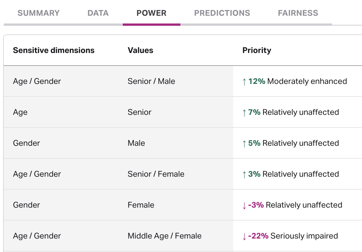
The level is also determined by relative_f1 according to the following rules:

• seriously_impaired: relative_f1 $< -0.2$
• moderately_impaired: $-0.2 \le$ relative_f1 $< -0.1$
• relatively_unaffected: $-0.1 \le$ relative_f1 $< 0.1$
• moderately_enhanced: $0.1 \le$ relative_f1 $< 0.2$
• seriously_enhanced: $0.2 \le$ relative_f1

Predictions

This category measures the proportion of a subpopulation $S$ in the target population $T$ against the baseline proportion in order to see if the subpopulation is over or under-represented.

The API response for predictions as part of an outcome analysis request has a similar structure to power (above) where dimensions and values determine $S$:

"dimensions": ["Age", "Gender"],
"values": ["Senior", "Male"]

along with an array of metrics:

"metrics": [
  {
    "name": "relative_odds_ratio",
    "level": "strong_bias",
    "value": 1.7344333595141825
  },
  {
    "name": "odds_ratio",
    "level": "strong_bias",
    "value": 2.7344333595141825
  }
]

The odds-ratio is defined by:

where $S$ denotes the subpopulation of interest, $T$ denotes the target population (in this case the top 5%), $E$ denotes the eligible population, and $|A|$ denotes the cardinality of a set $A$.

The relative odds-ratio is recentered at zero via relative_odds_ratio $= 1-$ odds_ratio.

The subpopulations in the API response are ordered by relative_odds_ratio (descending) and this value is also shown in the UI.

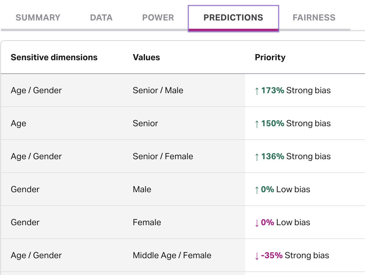
Let $m$ be the absolute value of relative_odds_ratio. Then a level of low_bias means $m\in[0, 0.1)$, moderate_bias means $m\in[0.1, 0.2)$, and strong_bias means $m\in[0.2, \infty)$.

Fairness

This category is concerned with reporting overall measures of fairness from the literature and combining them into a Faraday-specific fairness metric.

The API response for fairness as part of an outcome analysis request has a similar structure to power and predictions (above) where dimensions and values determine $S$

"dimensions": ["Age"],
"values": ["Senior"]

along with an array of metrics:

"metrics": [
  {
    "name": "relative_total_fairness",
    "level": "equitably_treated",
    "value": -0.16173819203227446
  },
  {
    "name": "total_fairness",
    "level": "equitably_treated",
    "value": -0.6469527681290979
  },
  {
    "name": "statistical_parity_difference",
    "level": "moderately_underprivileged",
    "value": -0.39568528261182057
  },
  {
    "name": "equal_opportunity_difference",
    "level": "equitably_treated",
    "value": 0.20719947839813313
  },
  {
    "name": "average_odds_difference",
    "level": "equitably_treated",
    "value": 0.16539421297112872
  },
  {
    "name": "disparate_impact",
    "level": "seriously_underprivileged",
    "value": 0.3761388231134608
  },
  {
    "name": "scaled_disparate_impact",
    "level": "moderately_underprivileged",
    "value": -0.6238611768865392
  }
]

statistical_parity_difference, equal_opportunity_difference, average_odds_difference, and disparate_impact were defined previously. scaled_disparate_impact is a transformed version of disparate_impact obtained by post-composing with the map:

We now define total_fairness as the sum of statistical_parity_difference, equal_opportunity_difference, average_odds_difference, and scaled_disparate_impact. Since these metrics all take values in $[-1,1]$ and are centered at $0$, their scales are comparable which allows us to compute relative_total_fairness as total_fairness divided by 4.

The subpopulations in the API response are ordered by relative_total_fairness (descending) and this value is also shown in the UI.

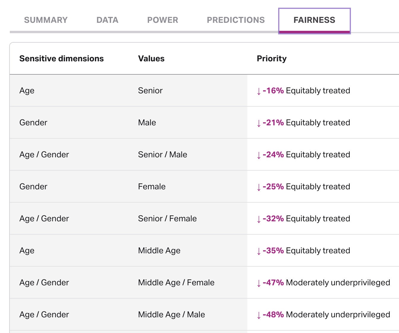
The level in the UI is determined by total_fairness and a value $\delta$ defined by:

Setting $\text{target rate} = 0.05$ (top 5%), we get $\delta = 1.\overline{45}$. Finally, the level shown in the UI is determined as follows:

• seriously_underprivileged: total_fairness $< -2\delta$
• moderately_underprivileged: $-2\delta\leq$ total_fairness $<-\delta$
• equitably_treated: $-\delta\leq$ total_fairness $<\delta$
• moderately_privileged: $\delta\leq$ total_fairness $<2\delta$
• seriously_privileged: $2\delta\leq$ total_fairness

Levels for individual fairness metrics returned via the API are documented in the API docs.

Calibration

Faraday outcomes are well-calibrated in the sense that an output score $f(x)$ is automatically transformed to approximate the probability $p(y=1\mid x)$. Currently, the calibration is a mapping of the form:

There are a number of benefits of having a calibrated outcome. The one that stands out in the context of this article is that the well-calibrated property implies that:

Thus, Faraday outcomes satisfy so-called test-fairness automatically from being well-calibrated.

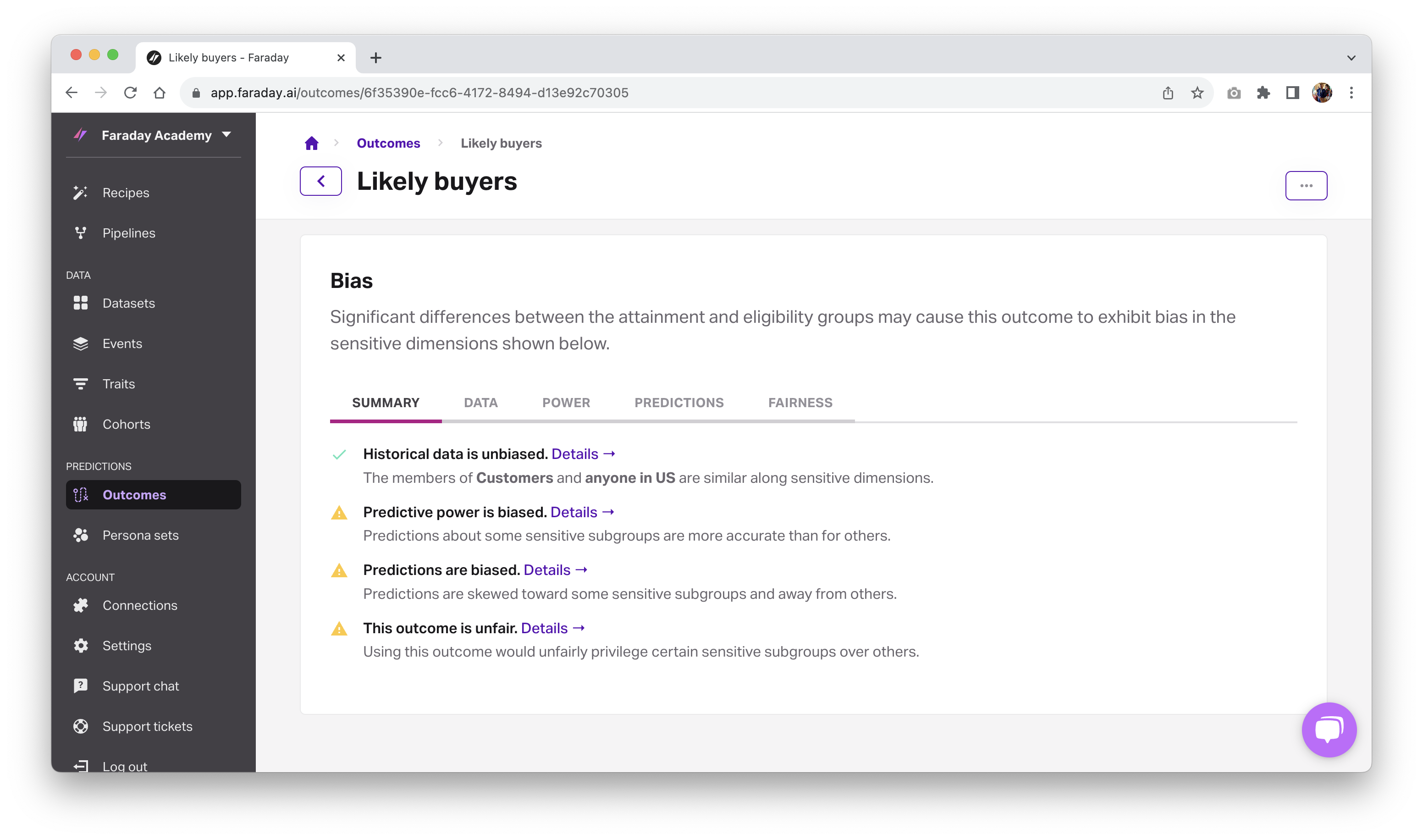
How to view bias in Faraday

The above examples detailing bias reporting were given in terms of the Faraday API, but these same metrics can also be accessed via the Faraday UI. When you navigate to the outcome you're interested in, scroll down to the bias section to see the breakdown of bias discovered in the data, power, predictions, and fairness categories detailed above.

Stay tuned for the followup blog post on mitigating bias with Faraday.

Ready to try Faraday? Create a free account.

References

[1] Mehrabi, N., Morstatter, F., Saxena, N., Lerman, K., & Galstyan, A. (2021). A survey on bias and fairness in machine learning. ACM computing surveys (CSUR), 54(6), 1-35.

[2] Max Hort, Zhenpeng Chen, Jie M. Zhang, Mark Harman, and Federica Sarro. 2023. Bias Mitigation for Machine Learning Classifiers: A Comprehensive Survey. ACM J. Responsib. Comput. Accepted (November 2023) original version 2018.

[3] Hardt, M., Price, E., & Srebro, N. (2016). Equality of opportunity in supervised learning. Advances in neural information processing systems, 29.

[4] Bellamy, R. K., Dey, K., Hind, M., Hoffman, S. C., Houde, S., Kannan, K., ... & Zhang, Y. (2019). AI Fairness 360: An extensible toolkit for detecting and mitigating algorithmic bias. IBM Journal of Research and Development, 63(4/5), 4-1.

[5] Garg, P., Villasenor, J., & Foggo, V. (2020, December). Fairness metrics: A comparative analysis. In 2020 IEEE International Conference on Big Data (Big Data) (pp. 3662-3666). IEEE.

[6] Verma, S., & Rubin, J. (2018, May). Fairness definitions explained. In Proceedings of the international workshop on software fairness (pp. 1-7).

[7] Dwork, C., Hardt, M., Pitassi, T., Reingold, O., & Zemel, R. (2012, January). Fairness through awareness. In Proceedings of the 3rd innovations in theoretical computer science conference (pp. 214-226).

[8] Kusner, M. J., Loftus, J., Russell, C., & Silva, R. (2017). Counterfactual fairness. Advances in neural information processing systems, 30.

[9] Ramdas, A., García Trillos, N., & Cuturi, M. (2017). On wasserstein two-sample testing and related families of nonparametric tests. Entropy, 19(2), 47.